Documentation
Here you can find the documentation of the services. Also read our Terms of Service.
1 Accessing the services
Our web services can be accessed via HTTP requests using the POST method Input arguments and parameters should be passed in a JSON format. The results are also returned in JSON. Please note, that for accessing the services the request should be made by using an API-Key, which is granted to the user after successful registration. The Key should be used in the x-api-key field of the request's header. Below in section 2 you can find some examples of defining such HTTP headers in various programming languages.
1.1 Model parameters
The service can be accessed via HTTP request using the URL:
https://lt-web.net/lactate/params
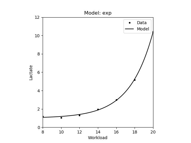
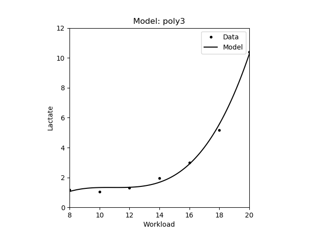
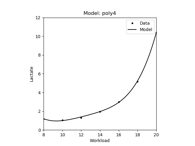
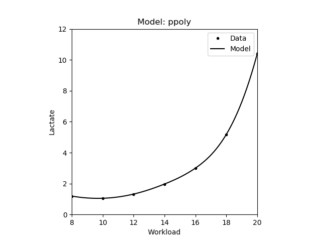
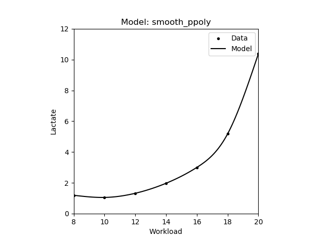
For determining the model parameters the following fields are mandatory in the JSON: workload, lactate, and func. Workload and lactate are lists of floating point numbers containing the measurement data. Func contains the identifier of the corresponding model. Currently the service provides the four models for estimating the lactate curve: exponential, 3rd and 4th degree polynomial, and piecewise polynomial by cubic spline fitting. A robust version of the 3rd degree polynomial is also available, which is more robust to outliers caused by corrupted lactate measurements. Note that the use of the robust version is not recommended for low sample size (e.g. less than 6 measurements). Also note that you can achieve a nearly perfect fit by piecewise regression, however it is not robust to noise. Thus it is not recommended when the number of noisy data points or outliers are high.
The JSON schema can be downloaded from here.
Below you can find some examples how your JSON should be created to access the service.| Model | Equation | JSON example | Plot |
|---|---|---|---|
| Exponential | \(y = b \times e^{cx} + a\) |
|
|
| 3rd degree polynomial | \(y = ax^3 + bx^2 + cx + d\) |
|
|
| 4th degree polynomial | \(y = ax^4 + bx^3 + cx^2 + dx + e\) |
|
|
| Robust 3rd degree polynomial | \(y = ax^3 + bx^2 + cx + d\) |
|

|
| Cubic Spline | Piecewise \(y = ax^3 + bx^2 + cx + d\) |
|
|
| Smooth Spline | Piecewise \(y = ax^3 + bx^2 + cx + d\) |
|
|
The result JSON contains the estimated model parameters in the params field in the same order as defined in the above table. The example below shows a JSON result for fitting an exponential model, thus the first params value in the returned JSON is the \(b\) of the exponential model \(y = b \times e^{cx} + a\). Additionally, in the fit_error field the error (namely the root mean squared error - RMSE) of the model fitting is returned. Note that a better fit usually results in a smaller error.
{
  "fit_error": 0.08790898569173469,
  "params": [0.003474546371577481,0.39500640217613003,1.0009130687036158]
}
In case of piecewise model fitting (spline or smoothing spline) the returned params are somewhat different. First, it contains intervals of the piecewise function in the intervals variable. Then the parameters of the polynomials are listed in the polys variable, namely for each polynomial defined at a given interval a separate params array is returned containing the coefficients of the corresponding polynomial. The type field describes the type of the individual piecewise functions (currently only 3rd order polynomials are supported). The example JSON below shows the result of a piecewise polynomial fitting.
{
  "fit_error": 4.652131608276905e-14,
  "params": {
    "intervals": [8.0,8.0,8.0,8.0,12.0,14.0,16.0,20.0,20.0,20.0,20.0],
    "polys": [
      {
        "params":[-5.952380952375299e-05,0.05303571428571254,-1.0101190476190298,5.907142857142798],
        "type":"poly"
      },
      {
        "params":[-5.952380952375299e-05,0.05303571428571254,-1.0101190476190298,5.907142857142798],
        "type":"poly"
      },
      {
        "params":[-5.952380952375299e-05,0.05303571428571254,-1.0101190476190298,5.907142857142798],
        "type":"poly"
      },
      {
        "params":[-5.952380952375299e-05,0.05303571428571254,-1.0101190476190298,5.907142857142798],
        "type":"poly"
      },
      {
        "params":[-0.0034523809523810817,0.17517857142857637,-2.4758333333333957,11.770000000000262],
        "type":"poly"
      },
      {
        "params":[0.013869047619047753,-0.5523214285714346,7.70916666666676,-35.76000000000046],
        "type":"poly"
      },
      {
        "params":[0.04422619047619044,-2.0094642857142837,31.02345238095234,-160.10285714285692],
        "type":"poly"
      },
      {
        "params":[0.04422619047619044,-2.0094642857142837,31.02345238095234,-160.10285714285686],
        "type":"poly"
      },
      {
        "params":[0.04422619047619044,-2.0094642857142837,31.02345238095234,-160.10285714285686],
        "type":"poly"
      },
      {
        "params":[0.04422619047619044,-2.0094642857142837,31.02345238095234,-160.10285714285686],
        "type":"poly"
      }]
  }
}
1.2 Aerobic thresholds - LTaer
Aerobic lactate threshold marks the upper limit of (nearly) exclusive aerobic metabolism, and allows low intensity workouts that can last hours. This intensity is also frequently called as lactate threshold. The service to estimate such thresholds can be accessed via HTTP request using the URL:
https://lt-web.net/lactate/ltaer
For determining the aerobic lactate threshold (LTaer) the following fields are mandatory in the JSON: workload, lactate, and method. Workload and lactate are lists of floating point numbers containing the measurement data. Method contains the identifier of the corresponding method. For most of the methods the lactate curve function (see 1.1) is also mandatory, and it should be defined in the func field.
The JSON schema can be downloaded from here.
The resulting JSON will contain the estimated aerobic threshold in the aer field. Note that there are cases when some methods do not have a solution. For example there is no guarantee that a lactate curve has an inflection point. In such cases the JSON result will contain a null. The example below shows the output of an aerobic threshold estimation.{
"aer": 13.428418224534179
}In the figures below the ★ symbol and red dotted lines will be used to denote the location of the corresponding threshold.
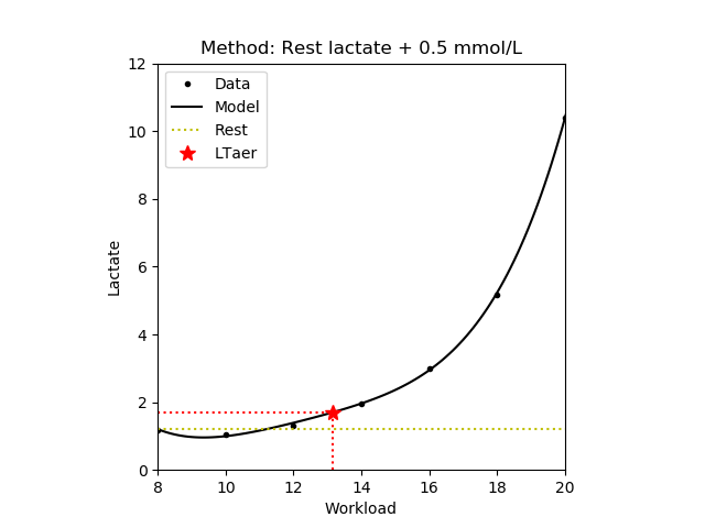
1.2.1 Rest
The workload where the blood lactate concentrate is 0.5 mmol/L above the resting lactate value [Hughson,1982]. Note that only those values are returned where the lactate concentrate is increasing. The figure below shows the estimated lactate threshold. The resting lactate is denoted by yellow dotted lines.
| JSON example | Plot |
|---|---|
|
|
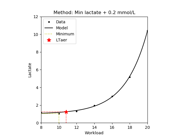
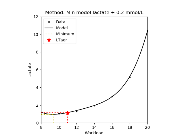
1.2.2 Workload minimum and Model minimum
The workload where the blood lactate concentrate is 0.2 mmol/L above the lowest lactate value (i.e. the lactate minimum) [Weltman,1988]. The minimum can be determined from the measured data (workload method) or from the estimated lactate curve (model minimum method). Note that only those values are returned where the lactate concentrate is increasing.
| Method | JSON example | Plot |
|---|---|---|
| Workload minimum |
|
|
| Model minimum |
|
|
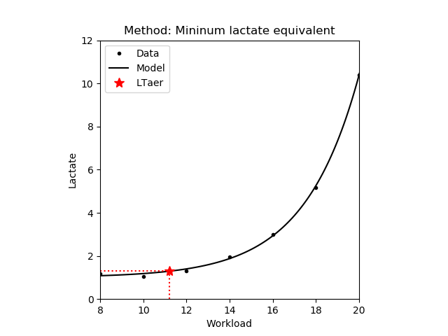
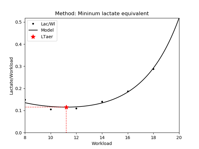
1.2.3 Minimum lactate equivalent (MLE)
The workload where the blood lactate concentrate divided by workload intensity takes its minima [Roecker,1998], [Dickhuth,1999]. Note that only those values are returned where the lactate concentrate is increasing.
| JSON example | Plot | Lactate/Workload |
|---|---|---|
|
|
|
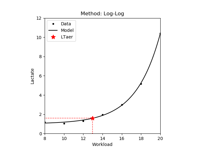
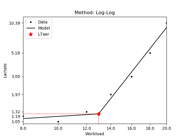
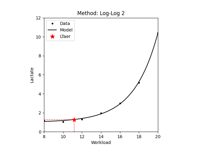
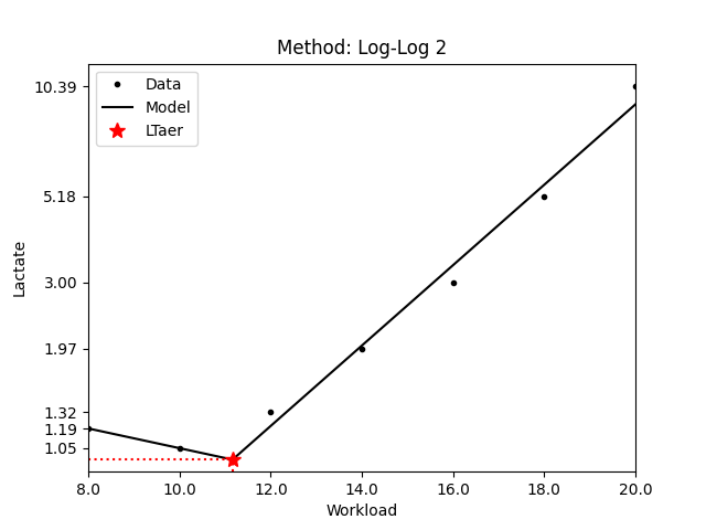
1.2.4 Log-Log
Assuming an exponential lactate curve, the Log-Log method fits a pairwise linear model on the logarithms of the workload intensity and the blood lactate. The threshold is determined as the intersection of the two regressed lines [Beaver,1985]. In the second variant (Log-log v2) the logarithm is applied to the lactate only.
| JSON example | Plot | Lines on log scale |
|---|---|---|
|
|
|
|
|
|
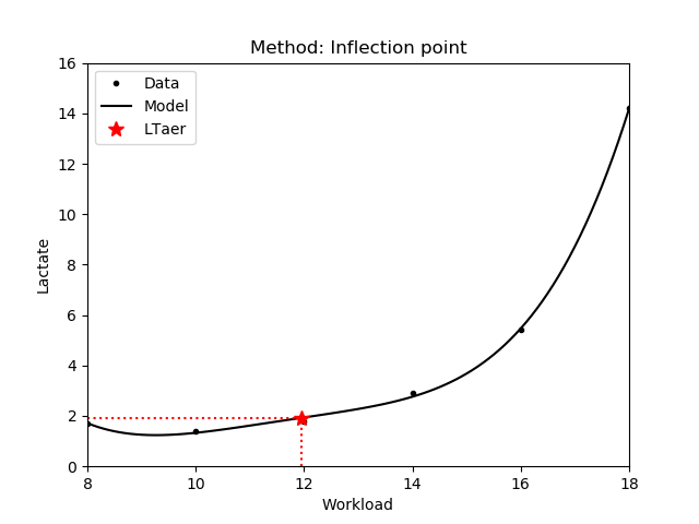
1.2.5 Inflection point
The workload where the lactate curve has an inflection point and it changes from concave to convex. This means that from this point the blood lactate concentrate increases exponentially with the workload intensity. Note that only those values are returned where the lactate concentrate is increasing. Also note that there is no guarantee that inflection point exists for a given lactate curve.
| JSON example | Plot |
|---|---|
|
|
Note that the exponential function does not have an inflection point, hence the func parameter should not contain the 'exp' model function (see 1.1).
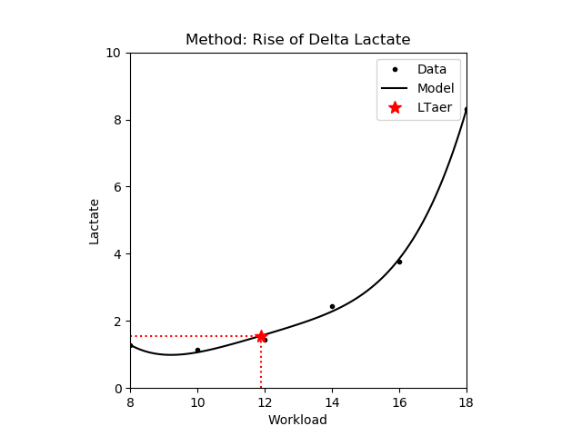
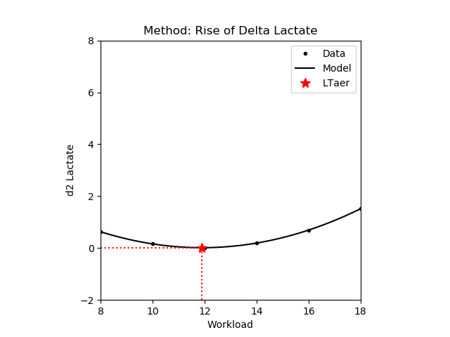
1.2.6 Rise of delta lactate
The workload where the accumulation of the blood lactate concentrate starts to rise exponentially with the intensity. In other words, it is equivalent to the workload where the rate of accumulation change reaches a minimum value. Note that only those values are returned where the lactate concentrate is increasing. Also note that it is equivalent to the inflection point if it exists. The use of this method is not recommended with piecewise polynomial model, as the minimum is usually equivalent with one of the interval points.
| JSON example | Plot | Rate of accumulation change |
|---|---|---|
|
|
|
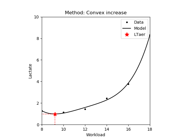
1.2.7 Convex increase
The workload intensity from where the blood lactate concentrate increases and the lactate curve is convex. In other words, the blood lactate increases faster than the workload intensity. Note that it is equivalent with the inflection point if it exists.
| JSON example | Plot |
|---|---|
|
|
Note that the exponential function will be convex and increasing from the starting point, hence using this method with the 'exp' model function is pointless.
1.3 Anaerobic thresholds - LTan
Anaerobic lactate threshold denotes the highest workload intensity where the blood lactate production and lactate elimination is in equilibrium, i.e. there is no blood lactate accumulation present. It is also commonly referred as maximal lactate steady state (MLSS) or lactate turnpoint. Workload intensities above this threshold are commonly used in interval trainings. Note that MLSS is the highest workload intensity that can be maintained over time without blood lactate accumulation, i.e. there is a balance between lactate production and clearance. On the other hand, anaerobic thresholds determined in incremental tests are generally used to estimate the MLSS intensity. The service can be accessed via HTTP request using the URL:
https://lt-web.net/lactate/ltan
For determining the anaerobic lactate threshold (LTan) the following fields are mandatory in the JSON: workload, lactate, and method. Workload and lactate are lists of floating point numbers containing the measurement data. Method contains the identifier of the corresponding method. For most of the methods the lactate curve function (see 1.1) is also mandatory, and it should be defined in the func field. Some of the methods also require the workload intensity at the aerobic threshold (see 1.2) as input parameter, and it should be defined in the aer_workload field of the JSON.
The JSON schema can be downloaded from here.
The resulting JSON will contain the estimated aerobic threshold in the an field. Note that similarly to the aerobic thresholds there are cases when some methods do not have a solution. In such cases the JSON result will contain a null. The example below shows the output of an aerobic threshold estimation.{
"an": 16.038469984768483
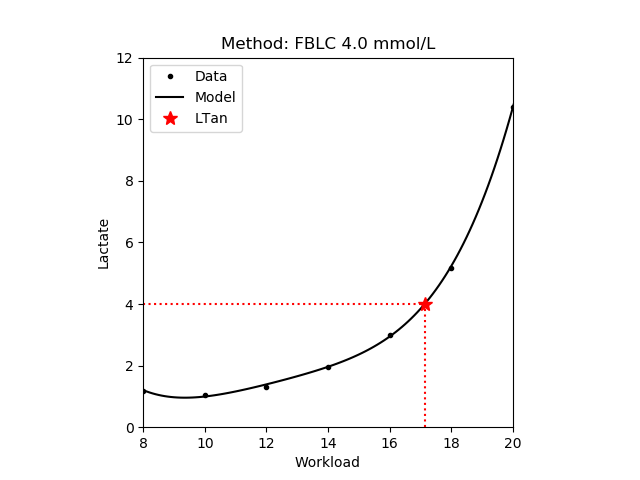
}1.3.1 Fix blood lactate concentrate - FBLC
The workload where the blood lactate concentrate reaches a fix 4.0 mmol/L value [Mader,1976]. This threshold is also known as onset of blood lactate accumulation (OBLA).
| JSON example | Plot |
|---|---|
|
|
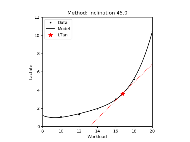
1.3.2 Inclination
The workload at a 51°34' inclination of the estimated lactate curve [Keul,1979]. In [Simon,1981] inclination of 45° is proposed. Note that in the figure below the red dotted line has an inclination of 45%. Also note that the above values depend on the units and scales used for the lactate curve. For example the 51°34' is equivalent to a 1.26 mmol/L/km/h of blood lactate increase.
| JSON example | Plot |
|---|---|
|
|
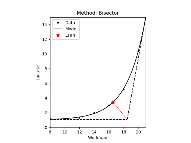
1.3.3 Bisecting tangents
The workload where the lactate curve intersects the bisecting line of the angle formed by the tangents at the lowest point of the curve and at the point equivalent to 15.0 mmol/L of blood lactate [Bunc,1986]. Note that similarly to the inclination (i.e. tangent) based methods, the bisecting angle and thereby the intersection with the lactate curve depends on the units and scale of the measurement data.
| JSON example | Plot |
|---|---|
|
|
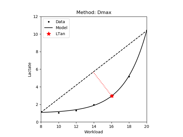
1.3.4 Maximum Distance - Dmax
The workload where the perpendicular distance of the lactate curve from the line defined by the start and endpoints of the lactate curve are maximal [Cheng,1992]. Another variant of the method uses the first and last measured data points to define this line (Dmax v2). Note that there is very little difference between the two variants. In the figures below a dashed black line connects the start and endpoints, and the red dotted line is perpendicular to this line.
| JSON example | Plot |
|---|---|
|
|
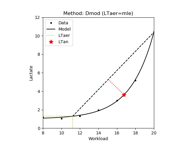
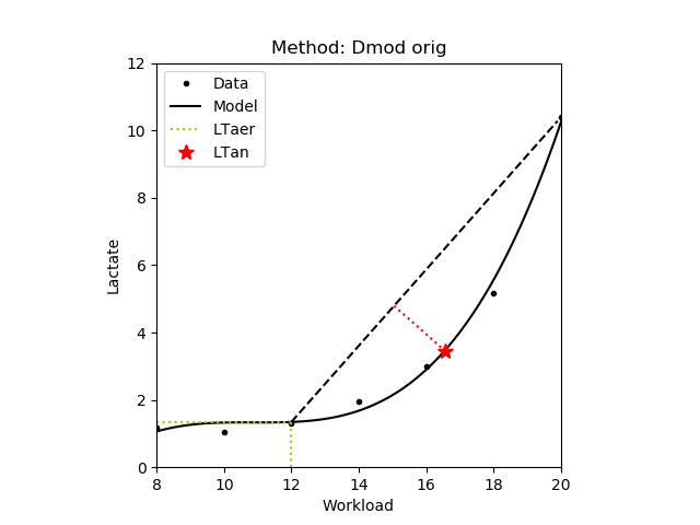
1.3.5 Modified Dmax - Dmod
A modification of the Dmax method (see 1.3.4) such that the startpoint of the line is the aerobic lactate threshold (see 1.2) [Bishop,1998]. The second variant uses last measured data point do define the line (Dmod v2). Finally, in the original method (Dmod orig) the startpoint is defined as the measurement that precedes an increase of at least 0.4 mmol/L [Bishop,1998]. Note that this point depends on the increments between the intervals, that is with larger increments the probability of observing such an increase is also larger. Also note that there is very little difference between the first and second variants. In the figures below the aerobic lactate threshold is denoted by yellow dotted lines.
| Method | JSON example | Plot |
|---|---|---|
| Dmod |
|
|
| Dmod orig |
|
|
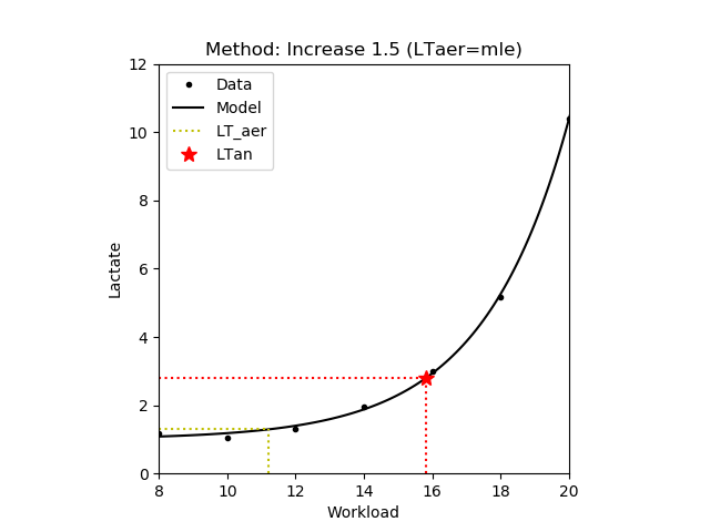
1.3.6 Increase
The workload at a blood lactate concentrate 1.5 mmol/L above the aerobic lactate threshold [Roecker,1998], [Dickhuth,1999]. In the figure below the aerobic lactate threshold is denoted by yellow dotted lines.
| JSON example | Plot |
|---|---|
|
|
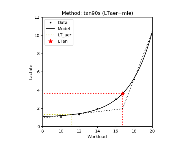
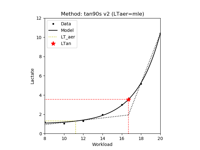
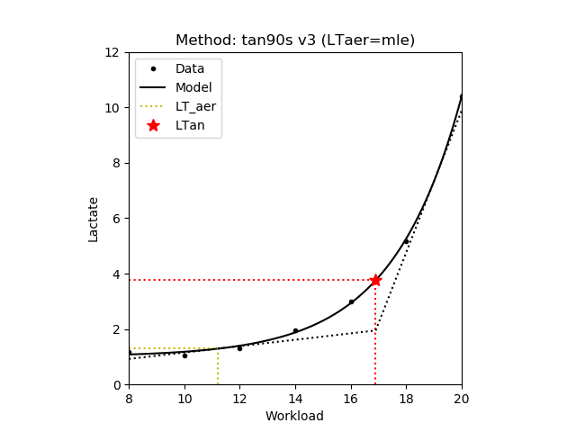
1.3.7 Tangent Intersections - Tan90s
The intersection point between the tangent at the aerobic lactate threshold and the linear function for the final 90 seconds of the incremental test (i.e. the last two lactate measurements) [Berg,1980]. In the second variant the values of the estimated lactate curve in the last two workload intensities are used to define the above linear function (Tan90s v2). Finally, in the third this line is defined as the tangential of the lactate curve having the inclination of the above line (Tan90s v3). Note that there is very little difference between the three variants. In the figure below the aerobic lactate threshold is denoted by yellow dotted lines. Additionally, the two lines are denoted by black dotted lines.
| Method | JSON example | Plot |
|---|---|---|
| Tan90s |
|
|
| Tan90s v2 |
|
|
| Tan90s v3 |
|
|
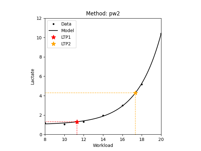
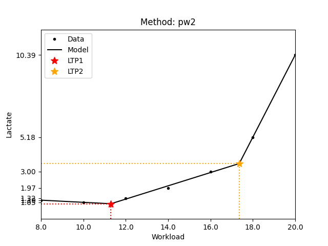
1.4 Lactate Turning Points - LTP1 and LTP2
This method assumes that the lactate curve can be divided into three segments, and each segment is represented by a linear function. The two lactate turning points (LTP1 and LTP2) are the intersections of the three segments. The service to estimate such thresholds can be accessed via HTTP request using the URL:
https://lt-web.net/lactate/ltp
For determining the lactate turning points the following fields are mandatory in the JSON: workload, lactate, and method. Workload and lactate are lists of floating point numbers containing the measurement data. Method contains the identifier of the corresponding method. Note that currently only the pw2 method is supported. The resulting JSON will contain the estimated turning points in the ltp1 and ltp2 fields. Note that there are cases when some methods do not have a solution. In such cases the JSON result will contain a null. The example below shows the output of a lactate turning point estimation.
{
  "ltp1": 11.292517006802727,
  "ltp2": 17.357742181540807
}| JSON example | Plot | Segments |
|---|---|---|
|
|
|
The parameters of the underlying piecewise linear model parameters can be accessed via HTTP request using the URL:
https://lt-web.net/lactate/pw2_params
The service returns the model as a piecewise linear (i.e. piecewise 1st degree polynomial - ppoly, see 1.1), which can be used in model evaluations (see 1.5).
1.5 Model evaluations
The service can be accessed via HTTP request using the URL:
https://lt-web.net/lactate/eval
For evaluating a model the following fields are mandatory in the JSON: params, func, and workload. Params contains the model parameters returned by the service described in 1.1, and it is either a list of floating point numbers (exponential or polynomial models), or the intervals and the list of polynomials (piecewise polynomials). Func contains the identifier of the corresponding model. Workload is a lists of floating point numbers containing the workloads where the model is evaluated.
The JSON schema can be downloaded from here.
The result JSON contains the model evaluations (i.e. the estimated lactate values) as a list of floating point numbers in the lactate field in the same order as the workload input. The example below shows a JSON result of an exponential model evaluated at 7 workload positions.
{
"lactate": [1.0828143919512172,1.1813764624934715,1.3985505571563053,
1.877077308198956,2.931474941668741,
5.254760666122612,10.373945673858907]
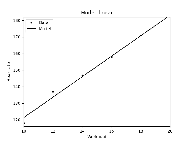
}1.6 Heart rate model parameters
The service can be accessed via HTTP request using the URL:
https://lt-web.net/lactate/hr_params
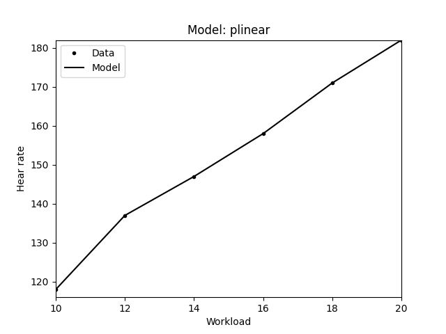
For determining the heart rate model parameters the following fields are mandatory in the JSON: workload, hr, and func. Workload and hr are lists of floating point numbers containing the measurement data. Func contains the identifier of the corresponding model. Currently the service provides two models for estimating the heart rate curve: linear and piecewise linear. Note that you can achieve a perfect fit by the piecewise linear, however it is not robust to noise.
The JSON schema can be downloaded from here.
Below you can find some examples how your JSON should be created to access the service.| Model | Equation | JSON example | Plot |
|---|---|---|---|
| Linear | \(y = m \times x + a\) |
|
|
| Piecewise Linear | Piecewise \(y = m \times x + a\) |
|
|
| Smooth Spline | Piecewise \(y = ax^3 + bx^2 + cx + d\) |
|
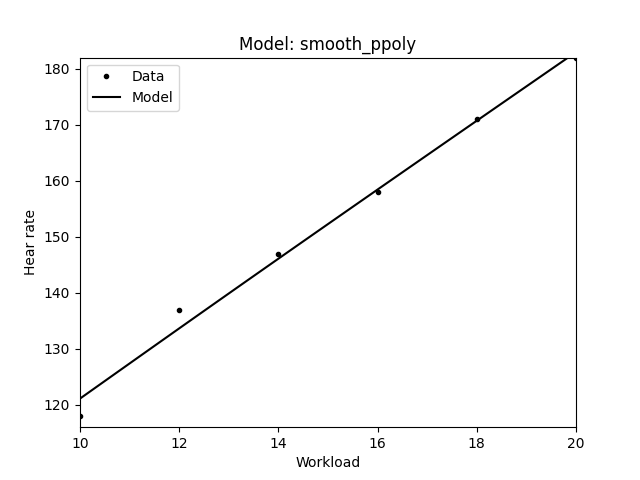
|
The result JSON contains the estimated hear rate model parameters in the params field in the same order as defined in the above table. The example below shows a JSON result for fitting a linear model, thus the first params value in the returned JSON is the \(m\) of the linear model \(y = m \times x + a\). Additionally, in the fit_error field the error (namely the root mean squared error - RMSE) of the model fitting is returned. Note that a better fit usually results in a smaller error.
{
  "fit_error": 2.0173847599903376,
  "params": [6.185714285714286,59.38095238095241]
}
In case of piecewise linear model fitting the returned params are somewhat different. First, it contains intervals of the piecewise function in the intervals variable. Then the parameters of the polynomials (linear functions) are listed in the polys variable, namely for each polynomial defined at a given interval a separate params array is returned containing the coefficients of the corresponding polynomial. The type field describes the type of the individual piecewise functions. The example JSON below shows the result of a piecewise linear fitting.
{
  "fit_error": 0.0,
  "params": {
    "intervals": [10.0,10.0,12.0,14.0,16.0,18.0,20.0,20.0],
    "polys": [
      {
        "params":[9.5,23.0],
        "type":"poly"
      },
      {
        "params":[9.5,23.0],
        "type":"poly"
      },
      {
        "params":[5.0,77.0],
        "type":"poly"
      },
      {
        "params":[5.5,70.0],
        "type":"poly"
      },
      {
        "params":[6.5,54.0],
        "type":"poly"
      },
      {
        "params":[5.5,72.0],
        "type":"poly"
      },
      {
        "params":[5.5,72.0],
        "type":"poly"
      }]
  }
}
1.6 Heart rate model evaluations
The service can be accessed via HTTP request using the URL:
https://lt-web.net/lactate/hr_eval
For evaluating a model the following fields are mandatory in the JSON: params, func, and workload. Params contains the model parameters returned by the service described in 1.5, and it is either a list of floating point numbers (linear model), or the intervals and the list of polynomials (piecewise linear model). Func contains the identifier of the corresponding model. Workload is a lists of floating point numbers containing the workloads where the model is evaluated.
The JSON schema can be downloaded from here.
The result JSON contains the model evaluations (i.e. the estimated heart rate values) as a list of floating point numbers in the hr field in the same order as the workload input. The example below shows a JSON result of a linear model evaluated at 6 workload positions.
{
  "hr": [121.23809523809527,133.60952380952384,
         145.98095238095243,158.352380952381,
         170.72380952380956,183.09523809523813]
}
2 Integration
Functions to make HTTP requests are offered in many software products and are available in most programming languages. Here you can find some examples of solutions for various tools such as Microsoft Excel, LibreOffice or Google Sheets. Note that the solutions below are provided "as is", meaning that we exclude all warranties.
2.1 Command line - curl
You can use curl to make HTTP requests from command line. curl is available for both Linux and Microsoft Windows. The example below demonstrates how to use curl to access the service from Windows command line.
curl.exe -k -H "Content-Type: application/json" -H "x-api-key: PUT-YOUR-API-KEY-HERE"
-X POST -d "{\"workload\":[8.0,10.0,12.0,14.0,16.0,18.0,20.0],\"lactate\":[1.19,1.05,1.32,1.97,3.0,5.18,10.39],
\"rest_lactate\":1.2,\"method\":\"rest\",\"func\":\"exp\"}" https://lt-web.net/lactate/ltaer
2.2 Microsoft Office Excel
In Excel you can make HTTP requests using Visual Basic macros.
Wl = "8.0,10.0,12.0,14.0,16.0,18.0,20.0"
Lac = "1.19,1.05,1.32,1.97,3.00,5.18,10.39"
Rest = "1.2"
method = "rest"
func = "exp"

Body = "{""workload"":[" & Wl & "],""lactate"":[" & Lac & "],""rest_lactate"":" & Rest &
       ",""method"":""" & method & """,""func"":""" & func & """}"

Set oHttp = CreateObject("MSXML2.ServerXMLHTTP")
oHttp.SetOption(2) = (oHttp.GetOption(2) - SXH_SERVER_CERT_IGNORE_ALL_SERVER_ERRORS)
oHttp.Open "POST", "https://lt-web.net/lactate/ltaer", False
oHttp.setRequestHeader "Content-type", "application/json"
oHttp.setRequestHeader "x-api-key", "PUT-YOUR-API-KEY-HERE"
oHttp.Send (Body)
response = oHttp.responseText

Set scriptControl = CreateObject("MSScriptControl.ScriptControl")
scriptControl.Language = "JScript"
Set jsonResponse = scriptControl.eval("(" + response + ")")
Please note that you may need to install additional libraries from Microsoft to access the above functionalities in Excel. The above example has been tested using Excel 2016 and Windows 10, and there is no guarantee that the code works with other versions without modifications. For example on the 64bit version of Excel the ScriptControl component is not available. In such cases you can use external VBA libraries (e.g. VBA-JSON), or follow the guidelines here.
2.3 LibreOffice Calc
LibreOffice macros can be written in various languages including Python. In Python you may use the requests package for making HTTP requests.
import requests
data = {
  'workload': [8.0,10.0,12.0,14.0,16.0,18.0,20.0],
  'lactate': [1.19,1.05,1.32,1.97,3.00,5.18,10.39],
  'rest_lactate': 1.2,
  'method': 'rest',
  'func': 'exp'
}
response = requests.post(
  https://lt-web.net/lactate/ltaer,
  json = data,
  headers = {
    'x-api-key': "PUT-YOUR-API-KEY-HERE"
  },
  verify = False
)
Please note that the default Python environment bundled with LibreOffice may not contain the requests and numpy, or other necessary packages by default. In such cases you need to install them manually. For example on Windows system the following commands can be used:
- Open command prompt as Administrator
- Change to LibreOffice directory, e.g. cd C:\Program Files\LibreOffice\program
- Download get-pip.py bootstrap script, e.g. c:\progs\curl-7.70.0-win64-mingw\bin\curl.exe https://bootstrap.pypa.io/get-pip.py -o get-pip.py
- Install pip: python.exe get-pip.py
- Install requests: python.exe -m pip install requests
- Install numpy: python.exe -m pip install numpy
- Changle LibreOffice macro security, e.g. in Calc Tools/Options/Security push the Macro Security button and change to Low
2.4 Google Sheets
Google Sheets uses JavaScript as macro language. The example below shows how to access the service.
var reqJson = {
  "workload": [8.0, 10.0, 12.0, 14.0, 16.0, 18.0, 20.0],
  "lactate": [1.19, 1.05, 1.32, 1.97, 3.00, 5.18, 10.39],
  "rest_lactate": 1.2,
  "method": "rest",
  "func": "exp"
};
var url = "https://lt-web.net/lactate/ltaer";
var headers = {
  'x-api-key': "PUT-YOUR-API-KEY-HERE"
};
var options = {
  'method' : 'post',
  'headers': headers,
  'contentType': 'application/json',
  'payload' : JSON.stringify(reqJson)
};
var response = UrlFetchApp.fetch(url, options);
var respJson = JSON.parse(response.getContentText());
return respJson;
3 References
| [Mader,1976] | Mader, A. et al., Zur Beurteilung der sportartspezifischen Ausdauerleistungsfähigkeit im Labor, Sportarzt Sportmedizin, 1976, 27: 80-88 und 109-112 |
|---|---|
| [Hughson,1976] | Hughson, R.L. and Green, H.J., Blood acid-base and lactate relationships studied by ramp work tests, Medicine and Science in Sports and Exercise, 1982, 14(4):297-302 |
| [Weltman,1988] | Weltman, A. et al., Prediction of lactate threshold and fixed blood lactate concentrations from 3200-m running performance in male runners, International Journal of Sports Medicine, 1988, 8(6):401-406 |
| [Roecker,1998] | Roecker, K. et al., Predicting competition performance in long-distance running by means of a treadmill test, Medicine and Science in Sports and Exercise, 1998, 30(10): 1552-7 |
| [Dickhuth,1999] | Dickhuth, H.H. et al., Ventilatory, lactate-derived and catecholamine thresholds during incremental treadmill running: relationship and reproducibility, International Journal of Sports Medicine, 1999, 20(2): 122-127 |
| [Beaver,1985] | Beaver, W.L. et al., Improved detection of lactate threshold during exercise using a log-log transformation, Journal of Applied Physiology, 1985, 59(6): 1936-1940 |
| [Keul,1979] | Keul, J. et al., Bestimmung der individuellen anaeroben Schwelle zur Leistungsbewertung und Trainingsgestaltung, Deutsche Zeitschrift für Sportmedizin, 1979, 30: 212-218 |
| [Simon,1981] | Simon, G. et al., Bestimmung der anaeroben Schwelle in Abhängigkeit von Alter und von der Leistungsfähigkeit, Deutsche Zeitschrift für Sportmedizin, 1981, 32: 7-14 |
| [Berg,1980] | Berg, A. et al., Zur Beurteilung der Leistungsfähigkeit und Belastbarkeit von Patienten mit coronarer Herzkrankheit, Deutsche Zeitschrift für Sportmedizin, 1980, 31: 199-205 |
| [Cheng,1992] | Cheng, B. et al., A new approach for the determination of ventilatory and lactate thresholds, International Journal of Sports Medicine, 1992, 13(7): 518-522 |
| [Bishop,1998] | Bishop, D. et al., The relationship between plasma lactate parameters, Wpeak and 1-h cycling performance in women, Medicine and Science in Sports and Exercise, 1998, 30(8): 1270-1275 |
| [Bunc,1986] | Bunc, V. et al., Determination of the individual anaerobic threshold, Acta Universitatis Carolinae Gymnica, 1985, 27: 73-81 |